NBA Calendar

Overview

As you might know (or not), NBA is the men’s professional basketball league in US. It contains 30 teams located around US and Canada (actually there is only one team in Canada) disputing the national title every year. If you have no idea about what I am saying maybe names such as Michael Jordan, Kobe Bryant, and Stephen Curry could help you. If still it does not sounds familiar this post probably will not be as delight as it is for me, but no problem we can still learn something from here.

The tournament is divided in two phases. First, these 30 teams play against each other during what is called the regular season. In the end of the regular season the best 8 teams from each conference (East and West) advance to the Playoffs where they dispute to be the Champion.

For my application, I will only focus on the regular season, when every team are playing against each other for a position in the Playoffs. During this period each team plays 82 games usually between October and April. Half of these 82 games are palyed at home and the other half is played away. It is very common for teams, during the regular season, have a sequence with more than one game away before playing at home, meaning they have to travel and stay away for more than one game.

For every regular season NBA defines a different calendar with time and location of the games. But this calendar cannot be randomly generate, otherwise we could end up with a very inefficient logistic calendar that would force teams to spend a lot of time and money on unnecessary trips. Moreover, this inefficient calendar could impact on the performance of the players.

Said that, it is plausible to claim that NBA already have an optmized regular season calendar. Where teams will not be playing away for a long period and also the amount of distance is minimized. They have an algorithm that create calendar subject to some constraints.

My point here is to explore the concept of Genetic Algorithm to create an efficient NBA calendar. Let’s see!!!

Load Necessary Functions

• collectNBACalendar: Function to download NBA calendar for a specific year.
• earth.dist: Given a pair of latitude and longitude calculate the distance between them.
• nbaFlightsByTeam: Returns a data frame with flights and the distance for a specific team during the season.

These functions were created from scratch to ease the porcess to manipulate data. More information about these functions can be found at my github account.

source('~/project/Data-Science-Projects/NBA calendar/NBA season calendar Functions.R')

Data

Scrapping data from internet

The data used are not in a well structured data frame. It was necessary to extract the calendar from internet. The function calendar is used to extract the nba calendar for an specific season.

Collecting the calendar from .

calendar<-collectNBACalendar(2016)

knitr::kable(head(calendar))

date	time	visitor	visitor_pts	home	home_pts	season
Fri, Jan 1, 2016	8:00 pm	New York Knicks	81	Chicago Bulls	108	2016
Fri, Jan 1, 2016	10:30 pm	Philadelphia 76ers	84	Los Angeles Lakers	93	2016
Fri, Jan 1, 2016	7:30 pm	Dallas Mavericks	82	Miami Heat	106	2016
Fri, Jan 1, 2016	7:30 pm	Charlotte Hornets	94	Toronto Raptors	104	2016
Fri, Jan 1, 2016	7:00 pm	Orlando Magic	91	Washington Wizards	103	2016
Sat, Jan 2, 2016	3:00 pm	Brooklyn Nets	100	Boston Celtics	97	2016

Create date format variable

Fri, Jan 1, 2016 -> 01-01-2016

calendar$date2<-unlist(lapply(strsplit(gsub(",","",calendar$date)," "),function(x) paste(x[2:4],collapse = "-")))
calendar$date2<-as.Date(calendar$date2,"%b-%d-%Y")
calendar<-calendar%>%
  arrange(date2)


### Minimum and Maximum for date2
calendar%>%
    filter(complete.cases(.))%>%
    group_by()%>%
    summarise(min=min(date2),max=max(date2))

## # A tibble: 1 x 2
##   min        max       
##   <date>     <date>    
## 1 2015-10-27 2016-06-19

Filtering Regular Season Games

This calendar contains playoffs games and as I said before we are only interested on regular season games. Therefore, we have to filter the season games.

The 2015-16 season ranged from 10-27-2015 to 04-13-2016

calendar<-calendar%>%
            filter(date2<='2016-04-13')

Checking

Checking if every time has 82 games.

# Quick check: Every team must have 82 games
print(sapply(unique(calendar$home),
       function(x) calendar%>%
  filter((home==x | visitor==x))%>%
  nrow()))

##          Atlanta Hawks          Chicago Bulls  Golden State Warriors
##                     82                     82                     82
##         Boston Celtics          Brooklyn Nets        Detroit Pistons
##                     82                     82                     82
##        Houston Rockets     Los Angeles Lakers      Memphis Grizzlies
##                     82                     82                     82
##             Miami Heat        Milwaukee Bucks  Oklahoma City Thunder
##                     82                     82                     82
##          Orlando Magic           Phoenix Suns Portland Trail Blazers
##                     82                     82                     82
##       Sacramento Kings        Toronto Raptors         Indiana Pacers
##                     82                     82                     82
##   Los Angeles Clippers        New York Knicks    Cleveland Cavaliers
##                     82                     82                     82
##         Denver Nuggets     Philadelphia 76ers      San Antonio Spurs
##                     82                     82                     82
##   New Orleans Pelicans     Washington Wizards      Charlotte Hornets
##                     82                     82                     82
## Minnesota Timberwolves       Dallas Mavericks              Utah Jazz
##                     82                     82                     82

Define Game Location

Based on the name of the home team we can identify the game location. For example, when the home team is ‘Chicago Bulls’ we know the game was hosted in Chicago.

In a simple example, for a match between ‘Chicago Bulls’ and ‘Memphis Grizzles’ where the home team is ‘Chicago Bulls’ we assume that there was travel from Memphis to Chicago.

# Home Location
calendar$home_location<-unlist(
  lapply(strsplit(calendar$home," "),
         function(x) paste(x[1:(length(x)-1)],collapse=" ")
         )
  )

# Visitor Location
calendar$visitor_location<-unlist(
  lapply(strsplit(calendar$visitor," "),
         function(x) paste(x[1:(length(x)-1)],collapse=" ")
         )
  )

Even though the code above was able to identify the games location we still had to do some manual adjustments.

For example:

• Golden State -> San Franciso (The team name does not contain the city’ name)
• Minnesota -> Minneapolis (The team name contains the state not the city name)

calendar$home_location[calendar$home_location=="Portland Trail"]<-"Portland"
calendar$home_location[calendar$home_location=="Utah"]<-"Salt Lake City"
calendar$home_location[calendar$home_location=="Indiana"]<-"Indianapolis"
calendar$home_location[calendar$home_location=="Minnesota"]<-"Minneapolis"
calendar$home_location[calendar$home_location=="Golden State"]<-"Oakland"
calendar$home_location[calendar$home_location=="Washington"]<-"Washington D.C."

Latitude and Longitude for the Cities where the Teams are located

Using the geocode function from ggmap package it is possible to download the latitude and longitude based on the city name.

#Example for Denver
geocode('Denver')

##         lon      lat
## 1 -104.9903 39.73924

Download for every team the latitude and longitude.

cities<-unique(calendar$home_location)
pos<-geocode(cities)
citiesLocation<-data.frame(cities,pos)

while(length(which(is.na(citiesLocation$lon)))>0){
 citiesLocation[which(is.na(citiesLocation$lon)),c("lon","lat")]<-geocode(cities[which(is.na(citiesLocation$lon))])
}

knitr::kable(head(citiesLocation))

cities	lon	lat
Atlanta	-84.38798	33.74900
Chicago	-87.62980	41.87811
Oakland	-122.27111	37.80436
Boston	-71.05888	42.36008
Brooklyn	-73.94416	40.67818
Detroit	-83.04575	42.33143

Calculate the Distance between Teams

The distance between any two cities is calculated by using its locations (latitude and longitude).

# Every combination between two teams
distance<-expand.grid(unique(calendar$home_location),unique(calendar$home_location))
names(distance)<-c("team1","team2")

# Join the location (latitude and longitude) for each team.
distance<-merge(x=distance,
                y=citiesLocation,
                by.x="team1",
                by.y="cities",
                all.x=TRUE)
names(distance)[3:4]<-c("lon1","lat1")

distance<-merge(x=distance,
                y=citiesLocation,
                by.x="team2",
                by.y="cities",
                all.x=TRUE)
names(distance)[5:6]<-c("lon2","lat2")

knitr::kable(head(distance))

team2	team1	lon1	lat1	lon2	lat2
Atlanta	Atlanta	-84.38798	33.74900	-84.38798	33.749
Atlanta	New York	-74.00597	40.71278	-84.38798	33.749
Atlanta	Denver	-104.99025	39.73924	-84.38798	33.749
Atlanta	Sacramento	-121.49440	38.58157	-84.38798	33.749
Atlanta	Phoenix	-112.07404	33.44838	-84.38798	33.749
Atlanta	Milwaukee	-87.90647	43.03890	-84.38798	33.749

Calculate the distance (km) between two cities using the function earth.dist.

distance$distance<-apply(
  distance[,names(distance)%in%c('lon1','lat1','lon2','lat2')],
  1,
  function(x) earth.dist(x[1],x[2],x[3],x[4],R=6378.145)
  )

knitr::kable(head(distance))

team2	team1	lon1	lat1	lon2	lat2	distance
Atlanta	Atlanta	-84.38798	33.74900	-84.38798	33.749	0.000
Atlanta	New York	-74.00597	40.71278	-84.38798	33.749	1201.662
Atlanta	Denver	-104.99025	39.73924	-84.38798	33.749	1949.539
Atlanta	Sacramento	-121.49440	38.58157	-84.38798	33.749	3354.758
Atlanta	Phoenix	-112.07404	33.44838	-84.38798	33.749	2559.549
Atlanta	Milwaukee	-87.90647	43.03890	-84.38798	33.749	1078.468

Function to calculate Distance traveled by a Team during the season

The nbaFlightsByTeam function returns a data frame with the flights and the distance for a specific team during the season.

For example for the Philadelphia 76ers

PHI_flights<-nbaFlightsByTeam(calendar,"Philadelphia 76ers",date=TRUE)
head(PHI_flights)

##    flight_from    flight_to  distance
## 1 Philadelphia       Boston  436.1181
## 2       Boston Philadelphia  436.1181
## 3 Philadelphia Philadelphia    0.0000
## 4 Philadelphia    Milwaukee 1115.2003
## 5    Milwaukee    Cleveland  539.5069
## 6    Cleveland Philadelphia  576.9254

The first 6 games of the 2016 season for the Phildelphia 76ers are:

Away(A)-Home(H)-H-A-A-H

The Phildelphia 76ers plays its first game at Boston and goes back home to play the next two games. Then they fly to Milwaukee and after that they go to Cleveland before coming back home for another game.

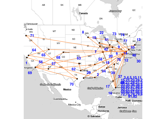
Philadelphia 76ers Travel Map

options(repr.plot.width=20, repr.plot.height=16)
nbaRouteMap(calendar,"Philadelphia 76ers")

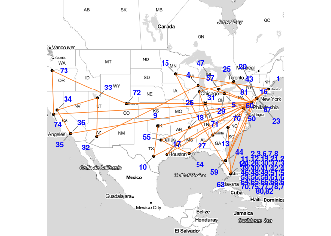
The blue numbers on the map represent the order of the games. The concentration of number on the bottom right are the home games.

To get the total kilometers traveled by the Philadelphia 76ers during the 2015-16 regular season we just have to sum the variable distance.

cat(format(sum(PHI_flights$distance),big.mark=",",scientific=FALSE),"km")

## 62,315.35 km

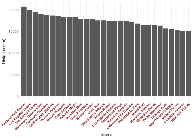
Total distance traveled by team during 2015-16 season

teams<-unique(calendar$home)
total_distance_by_team<-sapply(teams,function(x) sum(nbaFlightsByTeam(calendar,x)$distance))

total_distance_by_team<-as.data.frame(total_distance_by_team[order(total_distance_by_team,decreasing=TRUE)])
total_distance_by_team$team<-rownames(total_distance_by_team)
rownames(total_distance_by_team)<-NULL
colnames(total_distance_by_team)<-c('distance','team')
total_distance_by_team<-total_distance_by_team[c(2,1)]

options(repr.plot.width=8, repr.plot.height=4)
ggplot(total_distance_by_team,aes(x=reorder(team,-distance),distance))+
geom_bar(stat = "identity")+
theme_minimal()+
labs(x="Teams")+
labs(y="Distance (km)")+
 theme(axis.text.x = element_text(face="bold", color="#993333",
                           size=8, angle=45, hjust=1))

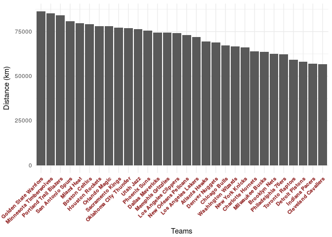
Interesting to see that both team that made NBA final are on the extrems. Coincidence?!? Yes, there is no correlation :P

Total distance traveled

If we sum the distance traveled by every team we have the total distance traveled during the season.

cat(format(sum(total_distance_by_team$distance),big.mark=",",scientific=FALSE),"km")

## 2,148,009 km

Propose a new calendar

If we shuffle the orders of the lines from the original calendar we can create a new calendar.

randomCalendar <- calendar[sample(nrow(calendar),replace=FALSE),]

Now, the first 10 games for Philadelphia 76ers using this new calendar would be:

randomCalendar%>%
select(home,visitor)%>%
filter(home=="Philadelphia 76ers" | visitor=="Philadelphia 76ers")%>%
head()

##                   home            visitor
## 1 New Orleans Pelicans Philadelphia 76ers
## 2   Philadelphia 76ers    Detroit Pistons
## 3      Milwaukee Bucks Philadelphia 76ers
## 4        Chicago Bulls Philadelphia 76ers
## 5   Philadelphia 76ers Washington Wizards
## 6   Philadelphia 76ers     Indiana Pacers

As you can see the total distance traveled by Philadelphia 76ers with this calendar has increased.

cat("Original Calendar:\t",
    format(sum(nbaFlightsByTeam(calendar,"Philadelphia 76ers",date=FALSE)$distance),big.mark=",",scientific=FALSE),
    "\nRandom Calendar:\t",format(sum(nbaFlightsByTeam(randomCalendar,"Philadelphia 76ers",date=FALSE)$distance),big.mark=",",scientific=FALSE))

## Original Calendar:    62,315.35
## Random Calendar:  101,729.5

Total distance traveled also has increased.

cat("Original Calendar:\t",
    format(sum(sapply(teams,function(x) sum(nbaFlightsByTeam(calendar,x,date=FALSE)$distance))),big.mark=",",scientific=FALSE),
        "\nCandidate Calendar:\t",
        format(sum(sapply(teams,function(x) sum(nbaFlightsByTeam(randomCalendar,x,date=FALSE)$distance))),big.mark=",",scientific=FALSE)
            )

## Original Calendar:    2,148,009
## Candidate Calendar:   3,178,847

How easy is to create a new calendar a with low distance traveled?

As I wrote in the begining of the post I believe it is hard to improve the original NBA calendar, but still we can try to create a new calendar with a resonable solution.

Let’s create 1,000 random calendars and check the distribution of the total distance traveled.

result<-rep(NA,1000)
for(i in 1:length(result)){
  c_<-calendar[sample(nrow(calendar),replace=FALSE),]
  result[i]<-sum(sapply(teams,function(x) sum(nbaFlightsByTeam(c_,x,date=FALSE)$distance)))
}

ggplot(data.frame(result),aes(x=result))+
  geom_histogram(fill="navy")+
  theme_minimal()+xlab("Distance (Km)")+ylab("")+
  geom_vline(xintercept = sum(sapply(teams,function(x) sum(nbaFlightsByTeam(calendar,x,date=TRUE)$distance))),colour="red",lty=2)

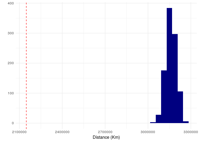
As we know the NBA Calendar has a total travel of 2,148,009 km (red dashed-line) and none of the 1,000 random calendars generate were closed to it. The minumum distance traveled generated from the 1,000 random calendars is greater than 3,000,000 Km. The original NBA calendar is really well optmized.

For this problem is possible to create 1230! different sequence of games. It is unfeasible to mannualy find a reasonable calendar by just generating a random sequence of games. The solution is to work with Genetic Algorithm to converge to an acceptable calendar.

Genetic Algorithm

There is no right answer for this problem. We are not looking for the best calendar, but one that might be a adequate. In this case we are looking for a calendar with a low distance traveled during the season.

This is an heuristic problem and can be solved by using the method so-called genetic algorithm (GA). The idea of this algorithm is pretty inspired by biological evolution (mutation, crossover and selection), that’s why the name genetic algorithm.

In a simple explanation, biological evolution are organisms reproducing and generating changes with each generation. In our case, organisms are the calendars and the evolution are a new calendars with changes generated from its ‘parents’ (previous calendars).

How it works?

If we have as initial calendar the random one we generated with a total distance traveled of 3,157,882 km. As we know that’s not a good calendar. The idea is to generated a new calendar from this one that could reduce this distance. One method to create this new calendar is randomly change some positions and check if it dereceased the total distance traveled. That’s the ideo of creating a new generation based on the previous one.

Let’s create 4 generations from our random calendar as first generation. In this process we proposed 10 random positions changes from this calendar and see the result.

random_distance<-sum(sapply(teams,function(x) sum(nbaFlightsByTeam(randomCalendar,x,date=FALSE)$distance)))

aux1<-randomCalendar

new_distance<-numeric(4)
new_distance[1]<-random_distance

#Create from 2nd to 4th generation
for(i in 2:4){
  new_distance[i]<-new_distance[(i-1)]+1
  while(new_distance[i]>new_distance[(i-1)]){
    for(j in 1:10){
      change<-sample(1:nrow(aux1),2,replace = TRUE)
      aux2<-aux1[change[1],]
      aux1[change[1],]<-aux1[change[2],]
      aux1[change[2],]<-aux2
      }
    new_distance[i]<-sum(sapply(teams,function(x) sum(nbaFlightsByTeam(aux1,x,date=FALSE)$distance)))
  }
}



cat("Distance First Generation Calendar:\t",
    format(random_distance,big.mark=",",scientific=FALSE),
    "\nDistance Second Generation Calendar:\t",
    format(new_distance[2],big.mark=",",scientific=FALSE),
    "\nDistance Third Generation Calendar:\t",
    format(new_distance[3],big.mark=",",scientific=FALSE),
    "\nDistance Fourth Generation Calendar:\t",
    format(new_distance[4],big.mark=",",scientific=FALSE)
    )

## Distance First Generation Calendar:   3,152,361
## Distance Second Generation Calendar:  3,129,660
## Distance Third Generation Calendar:   3,124,903
## Distance Fourth Generation Calendar:  3,113,575

In this simple example, each generation produced a lower total traveled distance calendar than its previous generation. If we keep running this procedure for further generations we could create a calendar with a similar distance from the original NBA calendar.

How to do it:

• Create 100 intial random calendars. It was created 100 so we can have more options.

• For each of the 100 calendars we create another calendar with a better result (lower total traveled distance) by changing positions. In this case we proposed initially 10 changes.

• From these 100 new calendars we select the top 60 with lower distance and randomly select 40 others (It will probably result in repeated calendars). This will select the best calendar and also randomly give a chance for others to present a better result in future generations.

• With these set of 100 calendars we repeat the whole process until we get a resonable result. In our case let’s use the total distance traveled in 2016 as reference (2,148,009 km).

Running the Genetic Algorithm from scratch

n_calendars<-100
#list_calendars<-list()
initial_n_changes<-2
n_interactions <- 230
modify_value <- 0
modify_check <- 0

n_changes<-10

# Initial 100 random calendars
for(i in 1:n_calendars){
  print(i)
  list_calendars[[i]]<-calendar[sample(1:nrow(calendar),nrow(calendar),replace = FALSE),]
  list_distance[[i]]<-sum(sapply(teams,function(x) sum(nbaFlightsByTeam(list_calendars[[i]],x,date=FALSE)$distance)))
}

# list of lists
list_calendars<-list(list_calendars)
list_distance<-list(list_distance)

# Create list for each interaction
aux_calendars<-list()
aux_distance<-list()


for(k in 1:n_interactions){
  print(paste0("************* Interaction = ",k," ***************"))

  # Select top 60 calendars + 40 random from every calendar
  candidates<-c(order(unlist(list_distance[[k]]))[1:60],sample(order(unlist(list_distance[[k]])),40,replace = TRUE))


  #### Update number of changes for each interaction ###

  if(modify_check>=50){
    modify_value <- modify_value+floor(modify_check/50)
    n_changes <- ifelse(modify_value>=initial_n_changes,2,initial_n_changes - modify_value)
  }
  else{
    n_changes <- initial_n_changes - modify_value
  }

  modify_check <- 0

  ####

  for(i in 1:length(candidates)){

    # Calculate the distance of the calendar that will be shuffled
    d<-sum(sapply(teams,function(x)
      sum(nbaFlightsByTeam(list_calendars[[k]][[candidates[i]]],x,date=FALSE)$distance)))

    # Variable for the new calendar distance. Intialize it longer than the current calendar
    new_d<-d+1

    # Counter
    count <- 0

    while(d<new_d && count<100 && n_changes!=0){
      aux1<-list_calendars[[k]][[candidates[i]]]
      print(paste0(i,"-",count," - changes: ",n_changes))
      for(j in 1:n_changes){
        change<-sample(1:nrow(aux1),2,replace = TRUE)
        aux2<-aux1[change[1],]
        aux1[change[1],]<-aux1[change[2],]
        aux1[change[2],]<-aux2
      }
      new_d<-sum(sapply(teams,function(x) sum(nbaFlightsByTeam(aux1,x,date=FALSE)$distance)))
      count<-count+1
      # If it takes more than 10 loops to find a better result
      if(count>=10 && count%%10==0){modify_check=modify_check+1}
    }

    aux_calendars[[i]]<-aux1
    aux_distance[[i]]<-new_d
  }

  # list of lists
  list_calendars[[k+1]]<-aux_calendars
  list_distance[[k+1]]<-aux_distance

  aux_calendars<-list()
  aux_distance<-list()

}

Taking the results

df<-as_tibble(
  do.call(cbind, lapply(list_distance,function(x) unlist(x)))
)

df$calendar<-1:nrow(df)

df<-melt(df,id=c("calendar"))%>%
  rename(interaction=variable)

data.frame(distance=map_dbl(lapply(
  list_distance,function(x) unlist(x)
),~quantile(.x,0.5)),
p5=map_dbl(lapply(
  list_distance,function(x) unlist(x)
),~quantile(.x,0.05)),
p95=map_dbl(lapply(
  list_distance,function(x) unlist(x)
),~quantile(.x,0.95)))%>%
  mutate(interaction=as.numeric(rownames(.)))%>%
  ggplot(aes(x=interaction,y=distance))+
  geom_line(col='navy')+
  geom_line(aes(x=interaction,y=p95),colour="orange")+
  geom_line(aes(x=interaction,y=p5),colour="orange")+
  theme_minimal()+
  geom_hline(yintercept = sum(sapply(teams,function(x) sum(nbaFlightsByTeam(calendar,x,date=FALSE)$distance))),colour="red",lty=2)

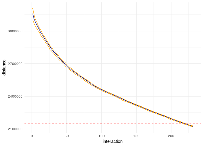
As we can see, after 200+ interactions we were able to generate a calendar with a lower distance than the 2016 calendar. The blue line represents the median of the 100 calendars and each yellow line represent 5% and 95% quantile of these 100 calendars.

The minimum distance traveled would be:

cat(format(sum(sapply(teams,function(x) sum(nbaFlightsByTeam(min_calendar,x,date = FALSE)$distance))),big.mark=",",scientific=FALSE),"km")

## 2,112,450 km

The total distance is obviously lower than the 2016 calendar. For this same calendar, the Philadelphia 76ers would travel:

cat("Original Calendar:\t",
    format(sum(nbaFlightsByTeam(calendar,"Philadelphia 76ers",date=FALSE)$distance),big.mark=",",scientific=FALSE),
    "\nNew Calendar:\t",format(sum(nbaFlightsByTeam(min_calendar,"Philadelphia 76ers",date=FALSE)$distance),big.mark=",",scientific=FALSE))

## Original Calendar:    62,315.35
## New Calendar:     67,528.54

It is actually more than the original calendar but it is not that different. It resulted in this map:

nbaRouteMap(min_calendar,"Philadelphia 76ers")

total_distance_by_team<-sapply(teams,function(x) sum(nbaFlightsByTeam(min_calendar,x,date = FALSE)$distance))

total_distance_by_team<-as.data.frame(total_distance_by_team[order(total_distance_by_team,decreasing=TRUE)])
total_distance_by_team$team<-rownames(total_distance_by_team)
rownames(total_distance_by_team)<-NULL
colnames(total_distance_by_team)<-c('distance','team')
total_distance_by_team<-total_distance_by_team[c(2,1)]

options(repr.plot.width=8, repr.plot.height=4)
ggplot(total_distance_by_team,aes(x=reorder(team,-distance),distance))+
geom_bar(stat = "identity")+
theme_minimal()+
labs(x="Teams")+
labs(y="Distance (km)")+
 theme(axis.text.x = element_text(face="bold", color="#993333",
                           size=8, angle=45, hjust=1))

In this scenario we would have Portland Trail Blazer with the most distance traveled. It seems to be reasonable given the location of Portland.

Discussion and Conclusion

Trying to randomly find a suitable calendar for NBA regular season seems to be almost an impossible mission. By using the idea of genetic algorithm we were able to create possible calendars that have a total distance traveled lower than real NBA calendars. One important limitation in this procedure is that we are not using any constraint. These calendars could easily be subject to some constraints such as maximum number of games away in a row or some special date games such as christmas and thanksgiving games. Applying these constraints would reduce the number of possible calendars and apparently would also make the process of finding a solution slower.